Show code to load packages
# Load packages
library(forecast)
library(tseries)
library(lubridate)
library(zoo)
library(xts)The previous section introduced a number of concepts that may have been new to you. In this section, we’ll introduce some further concepts and processes.
Again, try to grasp the concepts covered below. We’ll cover them in more detail during the practical session.
For TSA in R, it’s useful to have the following packages installed: forecast, tseries, lubridate, zoo and xts.
They all have different purposes and it’s good to know when to use which package!
# Load packages
library(forecast)
library(tseries)
library(lubridate)
library(zoo)
library(xts)Now, I’m going to create a synthetic dataset that we’ll use for the rest of the section.
In this dataset, we have one observation called value per month (date).
# Generate a Synthetic Time Series Dataset

# Set seed for reproducibility
set.seed(1234)

# Generate Date Sequence
start_date <- as.Date("2020-01-01")
end_date <- as.Date("2023-01-01")
dates <- seq.Date(start_date, end_date, by="month")

# Generate Synthetic Time Series Data
# We'll create data with a trend, seasonality, and random noise
trend <- seq_along(dates)
seasonality <- sin(seq_along(dates) * 2 * pi / 12) * 50 # Annual seasonality
noise <- rnorm(length(dates), mean = 0, sd = 5)

# Combine to Create Final Time Series Data
time_series_data <- round(trend + seasonality + noise,1)
time_series_data <- abs(time_series_data)

# Create a Data Frame
data <- data.frame(date = dates, value = time_series_data)

# Add Missing Values for Realism
set.seed(5678)
missing_indices <- sample(1:length(data$value), 5)
data$value[missing_indices] <- NA

# Clean environment

rm(dates, end_date, noise, seasonality, start_date, time_series_data, trend)

# Print head of the dataset
head(data,10)
date value
1 2020-01-01 20.0
2 2020-02-01 46.7
3 2020-03-01 58.4
4 2020-04-01 35.6
5 2020-05-01 32.1
6 2020-06-01 8.5
7 2020-07-01 20.9
8 2020-08-01 NA
9 2020-09-01 43.8
10 2020-10-01 37.8There may be missing data in the dataset. Remember, it’s important that we have equal numbers of observations in each time period (so for each year, at the monthly level, we need 12 observations).
For now, assume that this is the case. There are methods that we’ll learn about that can deal with missing observations in time-series data, but I’ll keep things simple at the moment.
# Check for missing values
missing_values_exist <- any(is.na(data$value))

missing_count <- sum(is.na(data$value))

print(paste("Number of missing values currently in data$value:", missing_count))
[1] "Number of missing values currently in data$value: 5"Simply deleting the 5 rows with missing data won’t work, because it will leave us with an unequal number of entries each year.
We need to use imputation instead.
Remember: Imputation is a technique used to handle missing data in datasets. When data points are missing, it can skew results and lead to inaccurate conclusions. Imputation involves filling in these missing values with substitutes, making the dataset complete for analysis. This substitution could be as simple as using the average or median of the available values.
# Handling missing values by imputing the mean value and replacing the missing value with the mean.
data$value[is.na(data$value)] <- mean(data$value, na.rm = TRUE) # Imputation
missing_values_exist <- any(is.na(data$value))
missing_count <- sum(is.na(data$value))
print(paste("There are now", missing_count, "missing values in data$value."))
[1] "There are now 0 missing values in data$value."rm(missing_count, missing_indices, missing_values_exist) # clear environmentAt the moment, R doesn’t know that this data is a time series. It just sees two columns of data.
To get things ready for time series analysis we can use a few different functions.
I’m going to start with ts, which is the most basic one. It’s good for monthly, quarterly and yearly data (but not so great for daily data).
To keep things very simple, I’m just going to delete the first column (date). ts only deals with one vector and can’t handle date and time information.
data_old <- data # I'm storing the original dataset in case I need it later

data$date <- NULL  # delete the `date` variable in `data`
To create a time series object in R using ts, we need to tell it at least one, but usually two things.
First, we need to define the frequency of our data.
If we have collected data monthly, the frequency is 12. We have twelve observations each year, each representing a month.
If we had collected data once every three months, our frequency would be 4 (4 observations per year).
We can also define what the start date of our time series is. In this case, it’s 2020,0 (the first observation in the series is the first month of the first year, 2020).
ts objsect# Creating ts Objects
ts_data <- ts(data$value, frequency=12, start(2020,0)) # For monthly data
print(ts_data) Jan Feb Mar Apr May Jun Jul Aug
1 20.00000 46.70000 58.40000 35.60000 32.10000 8.50000 20.90000 31.87187
2 34.10000 57.60000 69.80000 58.70000 39.40000 13.40000 10.20000 11.20000
3 31.87187 62.10000 79.90000 66.20000 31.87187 25.30000 11.50000 13.70000
4 51.10000
Sep Oct Nov Dec
1 43.80000 37.80000 16.40000 7.00000
2 31.87187 23.80000 4.20000 26.30000
3 20.50000 11.80000 1.90000 31.87187
4 Notice that the ts object ts_data now knows the time points of our observations. It knows that each observation represents a month, starting in January 2020.
We will return to this in more detail later. For now, just remember that we need to define this information in our time series object.
Now, we can get on with exploring our time-series. All of our analysis will take place on the ts_data time series.
From the previous section, you know that there are a number of things we want to focus on in time-series data. For now, we’re going to start with two of the most common exploratory techniques:
Time Series Plots: Creating line plots, scatter plots, and multiple time-series plots.
Seasonal and Trend Decomposition: Using decompose() and stl() functions.
Time-series plots are useful to explore trends or patterns in our data. For example:
# Time Series Plots
plot(ts_data)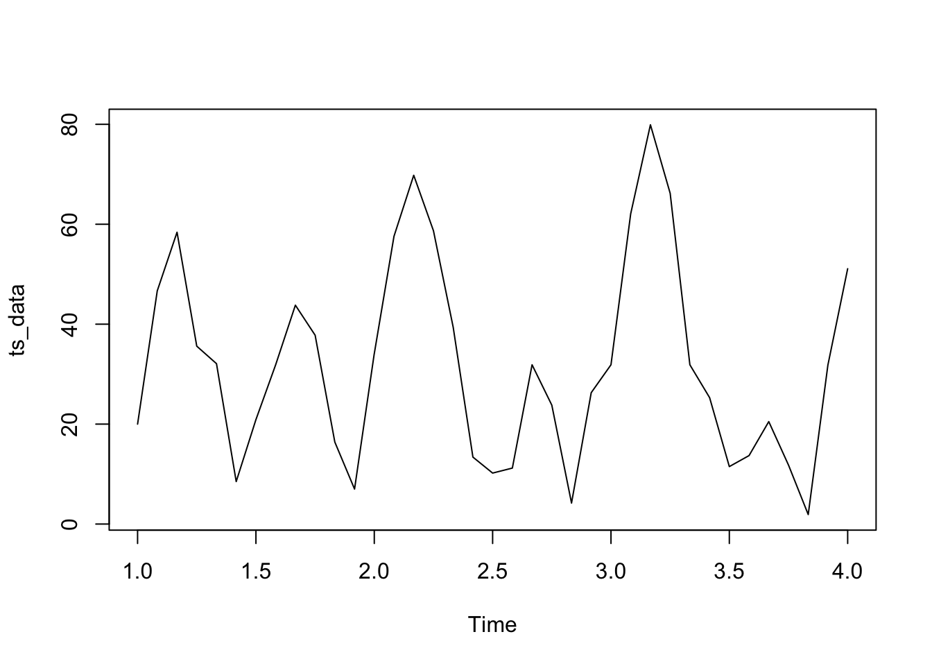
You’ll quickly see the weakness of this figure.
ts object doesn’t know how to allocate a date to each observation.The plot does give us a quick overview of the data, and the time points do align to the year (so 2.0 is the first month of 2021).
We can see, on initial inspection, that the data doesn’t have a clear trend; it goes ‘up and down’ over time.
It also appears that it tends to rise at the start of each year, and then drop down at the middle, then rise again towards the end of each year.
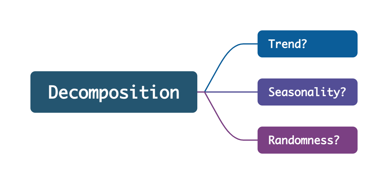
This next output is far more useful and is an example of decomposition.
Don’t worry too much about the detail for now, but what conclusions could you draw regarding trend and seasonality from this plot? Look at the seasonal row; what visual pattern can you identify that appears to be time-based?
# Seasonal and Trend Decomposition
decomposed_data <- decompose(ts_data)
plot(decomposed_data)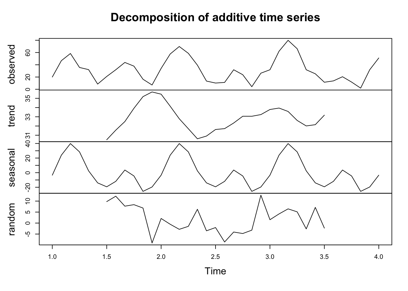
A lot of data we handle in sport is time-related. Therefore, it’s important to understand how R handles dates and times.
R primarily uses two classes to handle date and time data:
Date: for dates (year, month, day).POSIXct and POSIXlt: for date-time (date plus time of day).Let’s start by understanding how to work with these classes.
date classThe Date class is the simplest and is used to handle dates without time.
# Current date
today <- Sys.Date()
print(today)
[1] "2024-03-19"# Creating a Date object
specific_date <- as.Date("2021-12-31")
print(specific_date)[1] "2021-12-31"POSIXct and POSIXlt classesPOSIXct and POSIXlt are used for date-time data.
POSIXct represents the (date-time) as the number of seconds since the beginning of 1970 (known as the Unix epoch), whereas POSIXlt is a list that contains detailed information about the date-time.
# Current date-time
now <- Sys.time()
print(now)
[1] "2024-03-19 15:27:30 GMT"# Creating a POSIXct object
specific_datetime <- as.POSIXct("2021-12-31 23:59:59")
print(specific_datetime)[1] "2021-12-31 23:59:59 GMT"Using as.Date(), you can convert character strings to Date objects using as.Date().
# Convert a character string to a Date
date_from_string <- as.Date("2022-01-01", format="%Y-%m-%d")
print(date_from_string)
[1] "2022-01-01"Using as.POSIXct(), we can also work with date-time strings.
# Convert a character string to POSIXct
datetime_from_string <- as.POSIXct("2022-01-01 12:00:00", format="%Y-%m-%d %H:%M:%S")
print(datetime_from_string)
[1] "2022-01-01 12:00:00 GMT"Dates and times can come in various formats. It’s crucial to match the format in the as.Date() or as.POSIXct()functions.
# Different date format
date_euro_format <- as.Date("01/02/2022", format="%d/%m/%Y") # Day/Month/Year
print(date_euro_format)
[1] "2022-02-01"# Time in 12-hour format
datetime_12hr <- as.POSIXct("01/02/2022 01:30:00 PM", format="%d/%m/%Y %I:%M:%S %p")
print(datetime_12hr)[1] "2022-02-01 13:30:00 GMT"Sometimes you might want to extract the year, month, day etc., from an existing variable. This can be done as follows:
# Extracting components
year <- format(specific_datetime, "%Y")
month <- format(specific_datetime, "%m")
day <- format(specific_datetime, "%d")
hour <- format(specific_datetime, "%H")
minutes <- format(specific_datetime, "%M")
seconds <- format(specific_datetime, "%S")

print(paste("Year:", year, "- Month:", month, "- Day:", day, "- Hour:", hour, "- Minutes:", minutes, "- Seconds:", seconds))
[1] "Year: 2021 - Month: 12 - Day: 31 - Hour: 23 - Minutes: 59 - Seconds: 59"You can perform various operations like addition, subtraction, and difference calculation on date
Use base R operations to modify Date and POSIXct objects.
# Adding days to a date
future_date <- specific_date + 30
print(future_date)
[1] "2022-01-30"# Subtracting time from a datetime
past_datetime <- specific_datetime - as.difftime(1, units="hours")
print(past_datetime)[1] "2021-12-31 22:59:59 GMT"# Difference in days
date_diff <- as.Date("2022-02-01") - as.Date("2022-01-01")
print(date_diff)Time difference of 31 days# Difference in seconds
time_diff <- as.POSIXct("2022-01-01 13:00:00") - as.POSIXct("2022-01-01 12:00:00")
print(as.numeric(time_diff, units="secs"))[1] 3600Handling time zones in POSIXct is a critical aspect of date-time manipulation. This can be important if you’re working with data gathered from different countries.
# Creating a POSIXct object with a specific time zone
datetime_ny <- as.POSIXct("2022-01-01 12:00:00", tz="America/New_York")
datetime_london <- as.POSIXct("2022-01-01 12:00:00", tz="Europe/London")

# Comparing times
print(datetime_ny)
[1] "2022-01-01 12:00:00 EST"print(datetime_london)[1] "2022-01-01 12:00:00 GMT"lubridate Packagelubridate is a package that simplifies some common date-time operations.
# load lubridate
library(lubridate)

# Easy parsing of dates
ymd("20220101")
## [1] "2022-01-01"
mdy("01/02/2022")
## [1] "2022-01-02"
dmy("02-01-2022")
## [1] "2022-01-02"

# Arithmetic with lubridate
date1 <- ymd("2022-01-01")
date1 %m+% months(1) # Add a month
## [1] "2022-02-01"
date1 %m-% months(1) # Subtract a month
## [1] "2021-12-01"

# Extracting components
year(date1)
## [1] 2022
month(date1)
## [1] 1
day(date1)
## [1] 1Rounding off date and time to the nearest day, hour, etc.
# Rounding dates
round_date(datetime_ny, unit="day")
## [1] "2022-01-02 EST"
floor_date(datetime_ny, unit="hour")
## [1] "2022-01-01 12:00:00 EST"
ceiling_date(datetime_ny, unit="minute")
## [1] "2022-01-01 12:00:00 EST"Understanding the difference between duration (exact time spans) and period (human-readable time spans).
# Duration: exact time spans
duration_one_day <- ddays(1)
duration_one_hour <- dhours(1)
datetime_ny + duration_one_day
[1] "2022-01-02 12:00:00 EST"# Period: human-readable time spans
period_one_month <- months(1)
date1 + period_one_month[1] "2022-02-01"Handling Daylight Saving Time Dealing with complexities due to changes in daylight saving time.
# Before daylight saving time
dt1 <- as.POSIXct("2022-03-13 01:59:59", tz="America/New_York")

# After daylight saving time
dt2 <- dt1 + dhours(1)

print(dt1)
[1] "2022-03-13 01:59:59 EST"print(dt2)[1] "2022-03-13 03:59:59 EDT"